- Published at
Experiments with Sparse Autoencoders on Attention Heads
I trained sparse autoencoders on the key and query vectors of previous token heads and induction heads of attn-only-2l and gpt2-small and found interpretable features which I could intervene on in a predictable and interpretable way.
Note: This work was done in a two week research sprint as part of the MATS program
Summary
The main goal of this project was to apply sparse autoencoders to gain insight into the behaviour of several kinds of attention heads. To do this, I trained sparse autoencoders on the key and query vectors of previous token heads and induction heads of attn-only-2l and gpt2-small. The key findings are as follows:
- I found interpretable features in all of the attention heads. Between 20% and ~100% of alive features were interpretable, depending on the training parameters.
- In previous token heads, the features trained on query and key vectors are strongly dependent on the position within the context. In attn-only-2l, each feature corresponds almost exclusively to one position in the context. In gpt2-small, the positional dependence of each feature is spread more diffusively over 10 – 20 positions.
- In induction heads of attn-only-2l and gpt2-small, query and key features are usually of the form “I am [X]” and “I follow [X]” respectively, where [X] can be a single common token or a set of related less common tokens. The attention patterns can be well reproduced using these features. I found that I can causally intervene on the key vectors to delete “I follow ·D” such that induction on the token ·D no longer works.
- In some cases, I found that one feature accounted for ~90% of the probability assigned for the next token by the induction head despite an L0 norm of ~100, i.e. removing 99/100 activated features left the probability for the most common token mostly unchanged, and removing just the one strongest feature decreased the probability by a factor of 100. This suggests that the L0 norm may not be a good metric in certain situations.
- I could not identify a clear difference between the different induction heads in gpt2-small.
Motivation
Attention heads are difficult to understand yet are a critical component in understanding how LLMs work. Sparse autoencoders (SAEs) have been demonstrated to be useful tools in extracting features from MLP layers, both at mlp_post and mlp_out. Applying SAEs to attention heads might be a useful way to make it clear what they are doing. If I can improve or clarify the behaviour of attention heads that are already well understood, that would be a useful test of applying SAEs to attention heads. If I were able to use an SAE to show that an attention head does something that was not previously known about that attention head and that is difficult to show using other methods, that would be a good proof-of-concept for applying SAEs to attention heads.
Previous Token Heads
Attn-only-2l (L0H3)
Summary
| Metric | Query | Key |
|---|---|---|
| L0 Norm | 5.2 | 4.3 |
| Recovered loss | 97% | 92% |
| # Alive features | 250 | 256 |
| # Features | 256 | 256 |
| L1 coefficient | 0.03 | 0.03 |
- Trained an SAE on each of the query and key vectors
- Almost every query and key feature corresponds very strongly to one position in the context. Some correspond to two adjacent positions, and a small number (~10) are non positional dependent
- Query and key features can dot product to reproduce the previous token pattern i.e. query corresponding to position 40 dot products strongly with key corresponding to position 39 (see figure and discussion below)
- As an initial test, I set the context length to be 128 in the SAE training set and put 128 features in the SAE. Most of the features recovered in both the key and query SAEs correspond to particular directions. Because I didn’t recover a feature for all positions, I decided to run models with 256 features and a context length of 128. This recovered almost all of the positions (>120 out of 128).
- The attention pattern can be reconstructed based on the query and key vectors, and it works in combination with the induction head in the second layer of the two layer model.
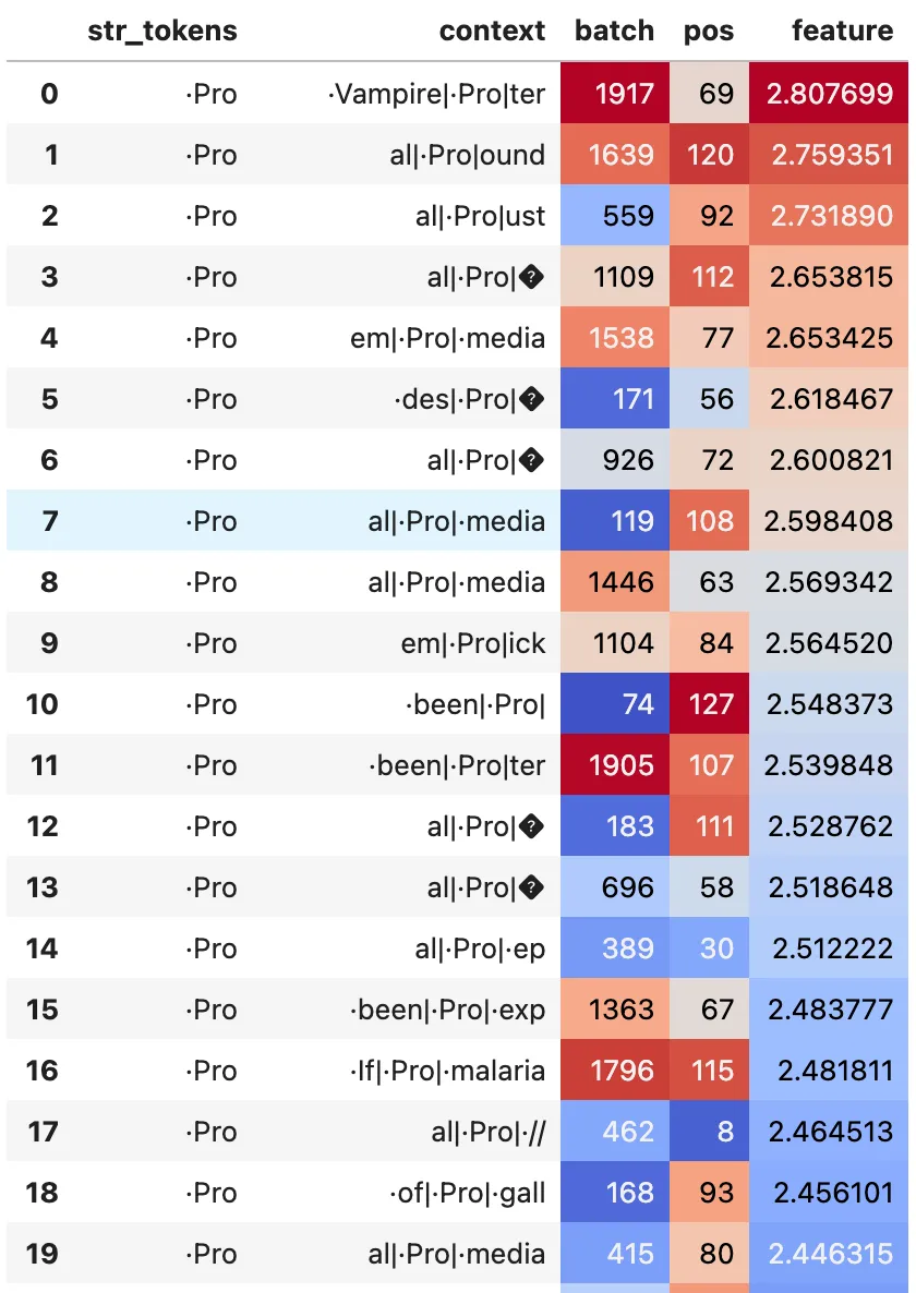
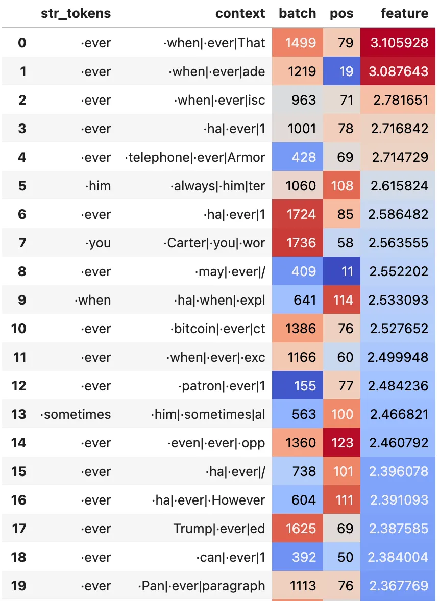
Typical Query Features
These are representative examples of max activations for two query features. Note that all the top 20 max activations are at the same position within a given feature. We can also see that there is some relatively weak token dependence of the feature activations.
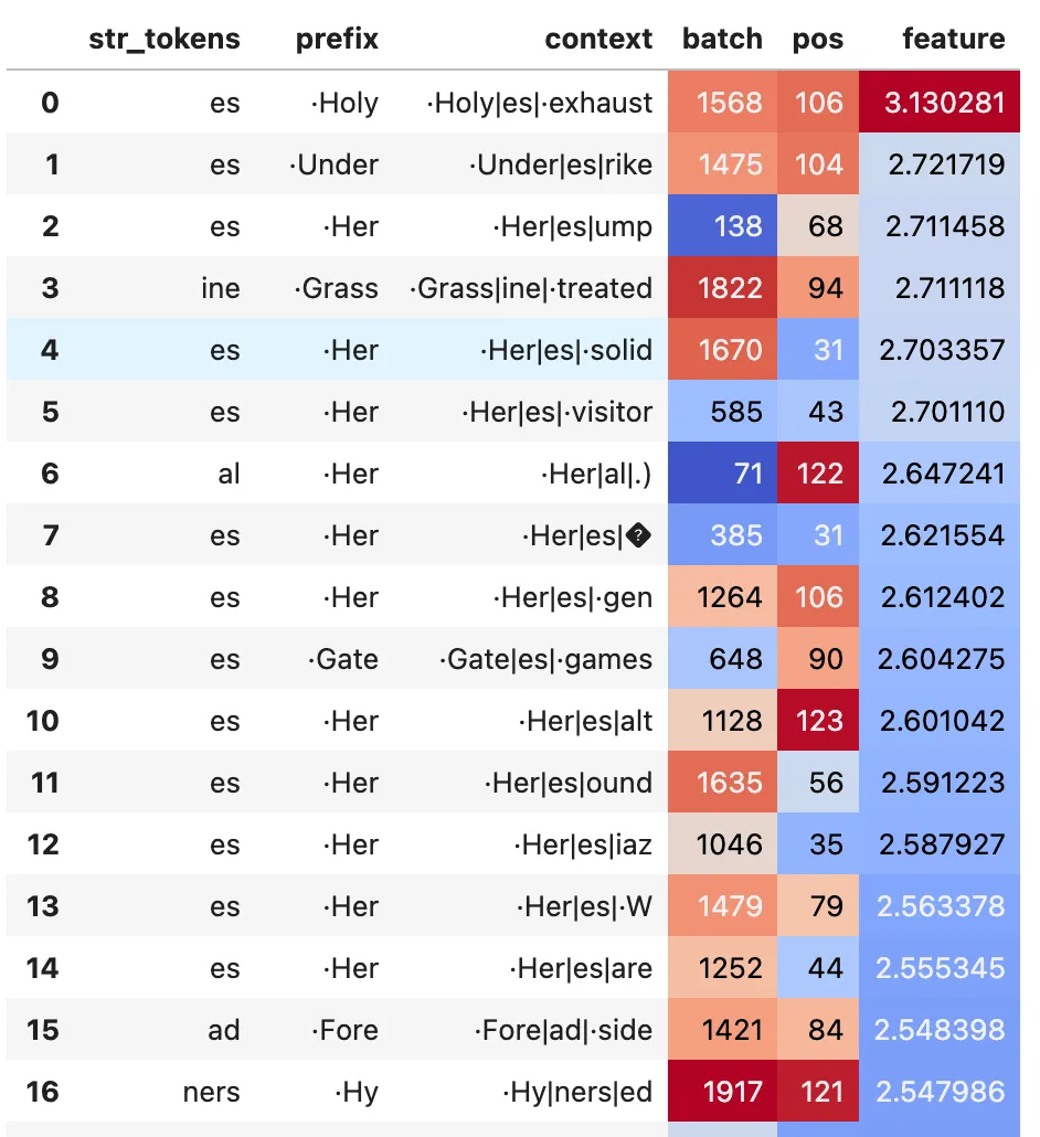
Typical Key Features
These are representative examples of max activations for two key features. Like the query features, all the top 20 max activations are at the same position within a given feature.
Positional Dependence of Features
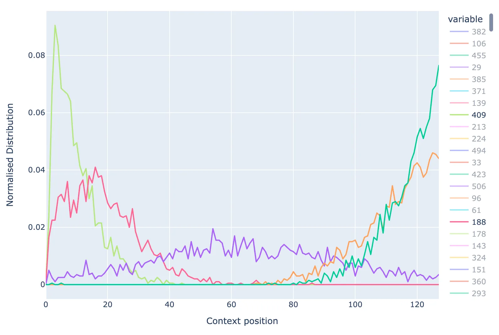
While the top 20 max activations for each query and key features have the same position in the context, one may wonder about the positions of the rest of the tokens on which a given feature activates (i.e. does query feature at position 40 also activate strongly for positions 39, for instance). To check this, I take the top 2000 max activating tokens (out of 500k, so ~4k per position) for each feature and plot the normalised distribution of the context positions. The figure below shows these position distributions for the query features. Only every 5th feature is plotted for clarity.
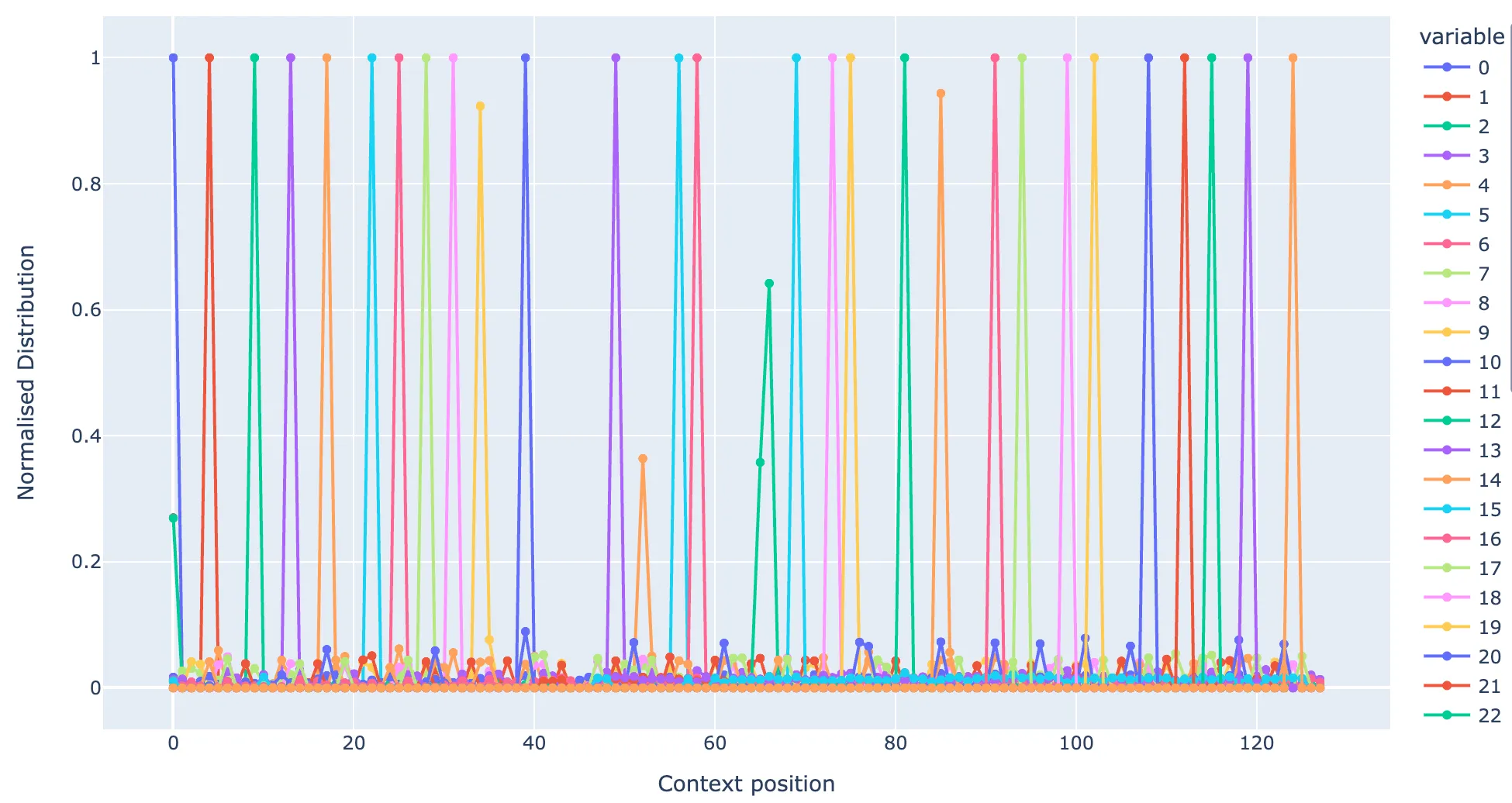
Distribution of the context positions of top 2000 max activating tokens per feature for SAE trained on previous token head.
We can notice that the majority of features have the same position at 100% of the top 2000 tokens (out of 500k, so ~4k per position). Some features have a roughly equal proportion of max activations at two adjacent positions, e.g. the dark green feature #15 at position ~65 in the figure. A small number of features are not dependent on position (see discussion in next subsection).
If you plot a similar positional dependence across the full data distribution (all 500k test tokens), each feature activates very weakly for a variety of other tokens. This appears to be related to the weak token dependence and is the reason the L0 norms are 5 and 4 for the query and key vectors respectively, rather than ~1 or ~2.
The same results are obtained for the features trained on the key vectors.
Non-Positional Features
While most of the features are positional based, there are some features that are token based. The figures below show one example. Key feature #120 fires on tokens that consist of subsets of words that are usually followed by a vowel, e.g ·qu, ·scr, ·gr, ·bl, ·sp ·st, ·sp, ·cr, ·cl (see max activations below). Out of the query features, key feature #120 has the largest dot product with query feature #133, the max activations of which are also shown below. Query feature #133 fires on tokens that consist of subsets of words beginning with vowels that one would typically find at the end of words and especially following the tokens that the key feature fires on e.g. ·ist, ·er, ·ed, ·ian, ·ant, ·ant (see max activations below). A next step to interpret this would be to train an SAE on the value vectors and see what is written out based on the attention constructed by these two features. But it’s clearly connecting together subsets of words. Note that while this is interesting to notice, in the case of attn-only-2l I think it is also possible to expand QK matrix pairs between all sets of tokens to achieve a similar result.
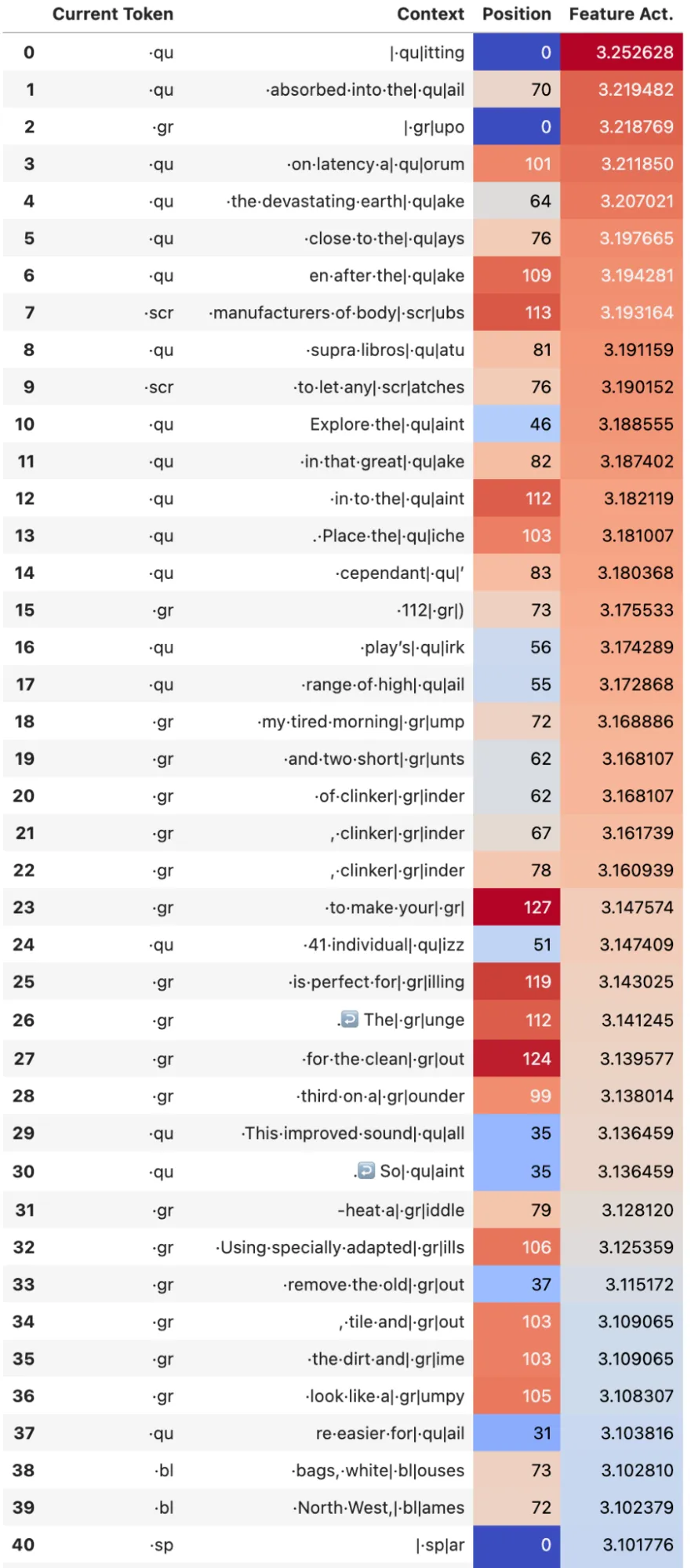
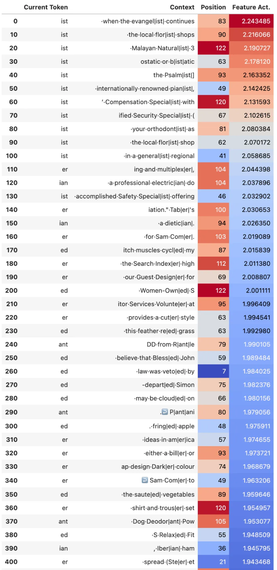
Max activating examples for non positional features in the previous token head. Left: Key Feature #120. Right: Query Feature #133
Reconstructed Attention Pattern
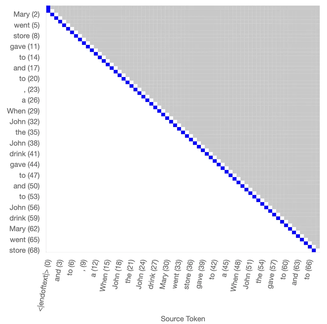
The attention pattern for the previous token head L0H3 can be reconstructed successfully using the key and query features across a range of tokens. Below is a visual example with the prompt “When Mary and John went to the store, John gave a drink to Mary”. The reconstructed pattern gets the positional dependence correct, and also does reasonably well for the weak token dependence. This reconstructed pattern can be connected with the induction head in layer 1 to perform induction successfully.
Original attention pattern Reconstructed attention pattern
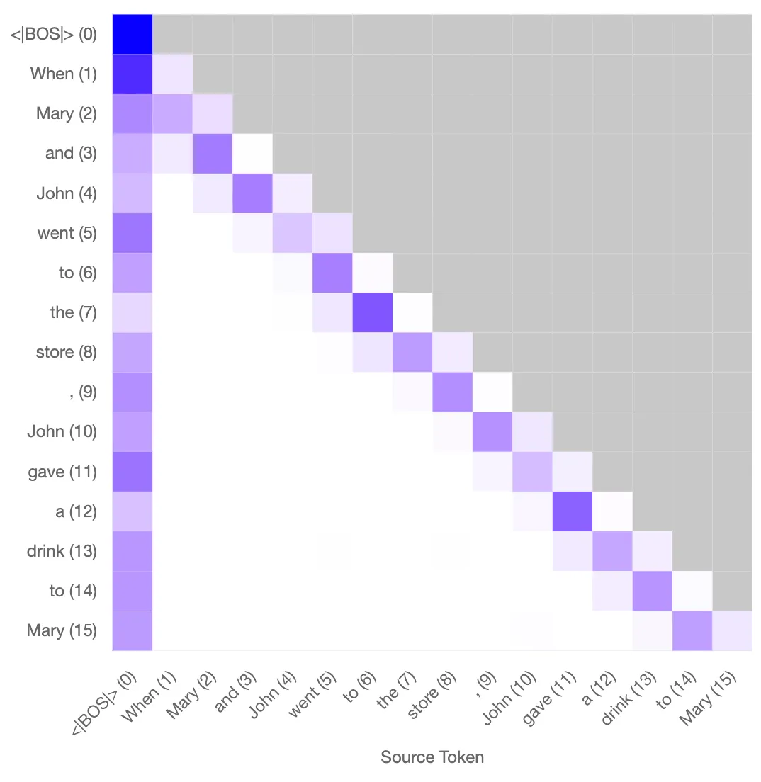
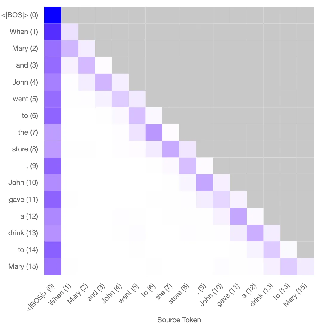
Left: Original attention pattern for the prvious token head. Right: Reconstructed attention pattern using the sparse autoencoder. This reconstructed pattern can combine with the induction head in L1 to perform induction.
Dot Product of Features sorted by Position
Since we have sets of key features and query features that correspond to one position in the context, one could imagine that the dot products between each key and query vector should reflect the behaviour of previous token heads. For instance, one might expect that the query feature that corresponds to position #20 should have the largest dot product with the key feature that corresponds to position #19.
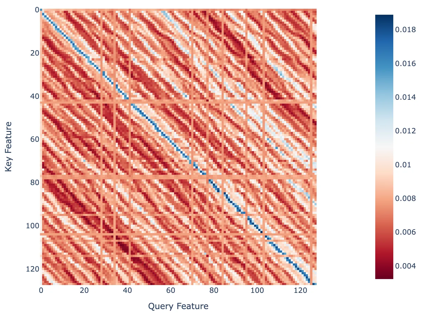
Dot product between a set of ~128 features from the query and key SAEs ordered by the position they correspond to.
The figure shows the dot product between a set of ~128 features from the query and key SAEs ordered by the position they correspond to. This simulates the attention scores between each feature. We can see that we recover the behaviour of a previous token head (the dark blue line is one below the main diagonal). The solid lines indicate context positions for which there is no single query or key feature corresponding to that position. These positions are represented by multiple features which allows the reconstructed attention pattern shown earlier to be correct.
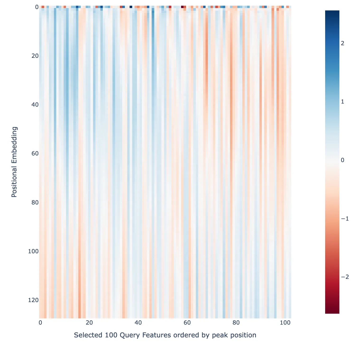
Dot Product of Features with Positional Embeddings
We can also check how the positional and key features that correspond to each position dot product with the positional embeddings of the model. The two figures below show such a calculation for the key and query features ordered by the position. The dark blue line is along the main diagonal indicating that the key and query features are picking up on the positional embeddings.
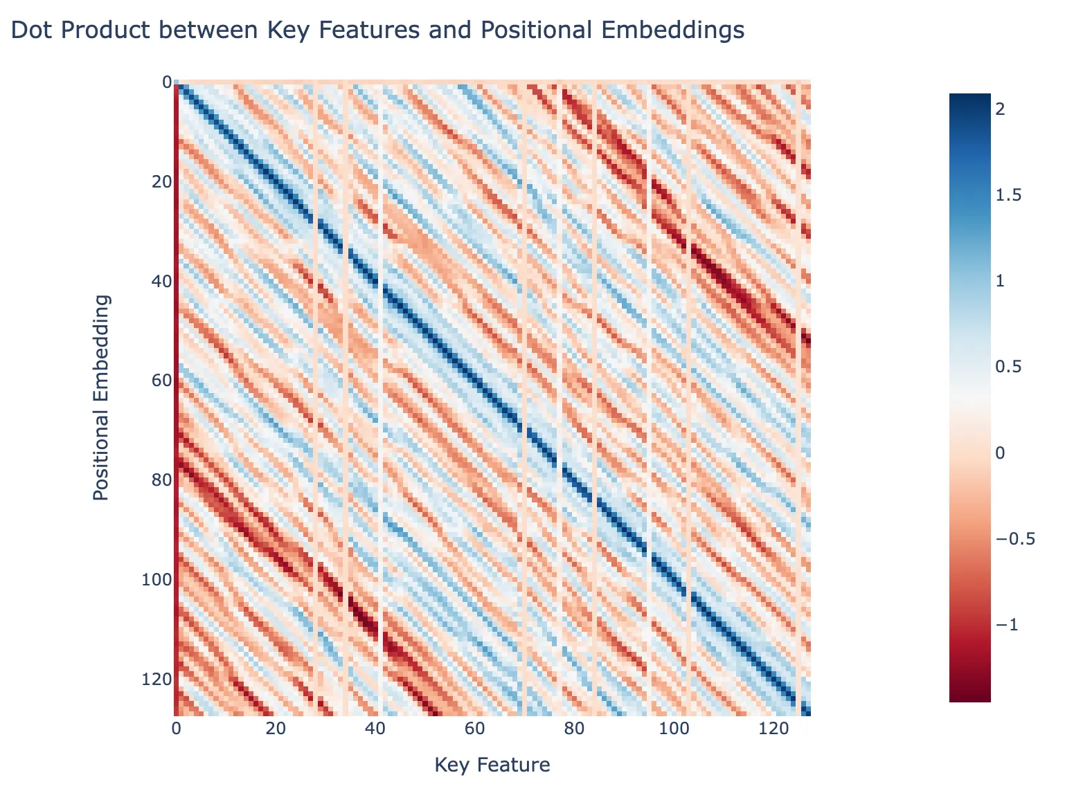
Dot product between Key Features and Positional Embeddings
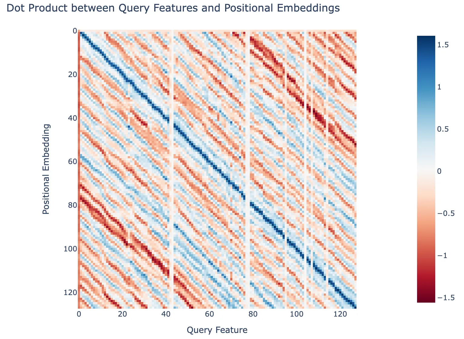
Dot product between Query Features and Positional Embeddings
GPT2-small (L4H11)
Summary
- I trained an SAE on the query and key features of the previous token head in gpt2-small.
- As I discuss below, both the key and query features are clearly related to position, but appear to be spread over many positions and there is no one-to-one correspondence between features and positions like there is in attn-only-2l. Clear features for positions 0 and 1 always show up, and sometimes for one or two other positions. But no matter which hyperparameters I chose, I could not replicate the figures from the previous token head for attn-only-2l.
- Despite this, the attention patterns can be reconstructed reasonably well
- I found it difficult to achieve a low L0 norm without totally killing the recovered loss. Possible solutions to this are to increase the number of features, train for longer or optimise for matching the attention pattern rather than loss. This is also a problem for other heads in gpt2-small.
- This is strange, but anecdotally query vectors seem easier to train on than key vectors across a few different heads that I looked at (are they less dense?)
- Also tried the same tests on L2H2, another previous token head in GPT2-small, and had similar results
Positional Dependence of Features
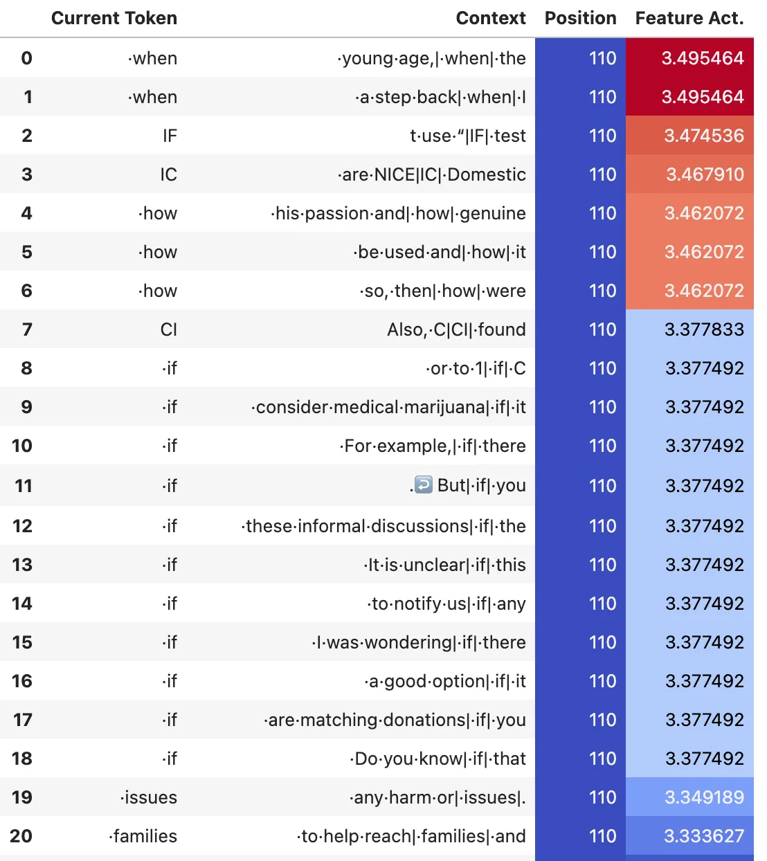
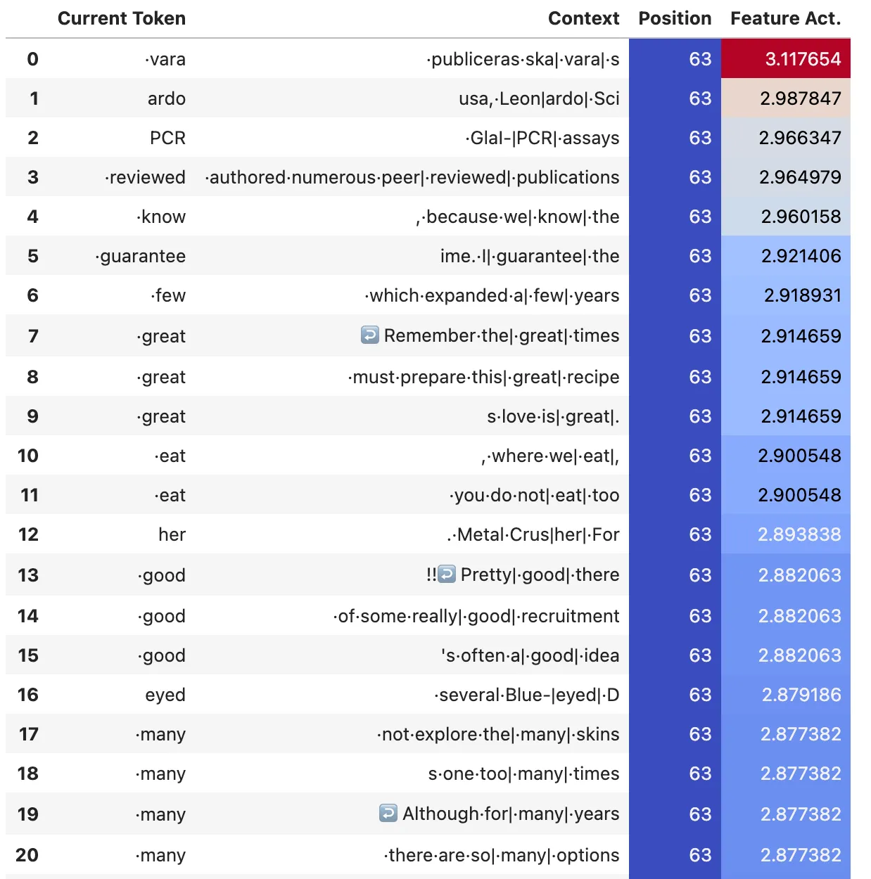
To look at the positional dependence of the features, I made a similar plot of the positional dependence of the features to the one from attn-only-2l. The below plot shows the normalised distribution of positions for five representative query features.
Distribution of positions of top 2000 max activating tokens for a five representative query features.
We can see that there is clearly a positional dependence, though it’s much more spread out in position than the features from the two layer model. I tried varying the SAE width (from 128 to 16384), the L1 coeff (from 0.0001 to 0.1), and training for longer (up to 500m activations), but could not yet find a combination that produced sharper distributions. I can’t figure out if they should exist or not. But I feel that with more time I could further optimise the SAE to verify this.
Dot Product of Features with positional embeddings
Since the features are much more spread out in position than in attn-only-2l, we might expect the dot products of the features with the positional embeddings to be similarly less sharp. This is indeed the case, as the following figure shows. It’s very spread out, but there is a weak correlation, i.e. blue in top left and bottom right.
Dot product between a set of ~128 features from the query and key SAEs ordered by the position they correspond to.
Reconstruction of features
The figure shows the reconstructed attention pattern for the previous token head based on the key and query vectors for a somewhat randomly chosen prompt of “When Mary and John went to the store, John gave a drink to” repeated 3 times. Despite the less sharp positional dependence of the features compared to the attn-only-2l model, the previous token head behaviour is recovered very well.
Reconstructed attention pattern for the previous token head based on the key and query vectors
Searching for features that impact attention scores
This is just an example of a simple method I used to find features that were actually affecting the attention score in a given context (as opposed to the feature activations on a given token which are not always the same as those that give the largest dot product). There is no significant conclusion from this subsection, just something I found useful.
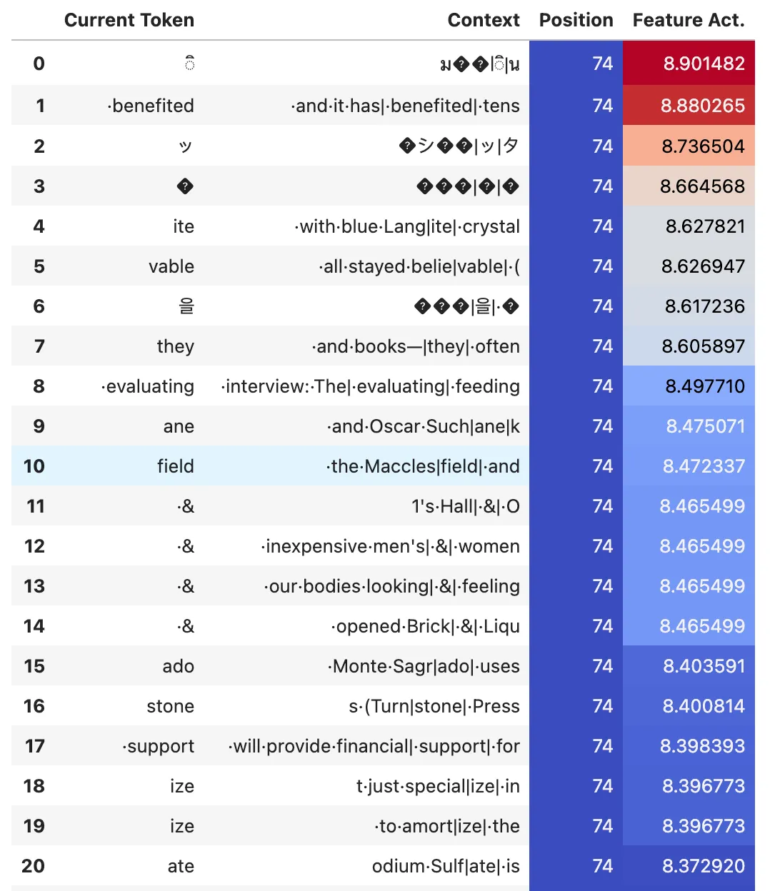
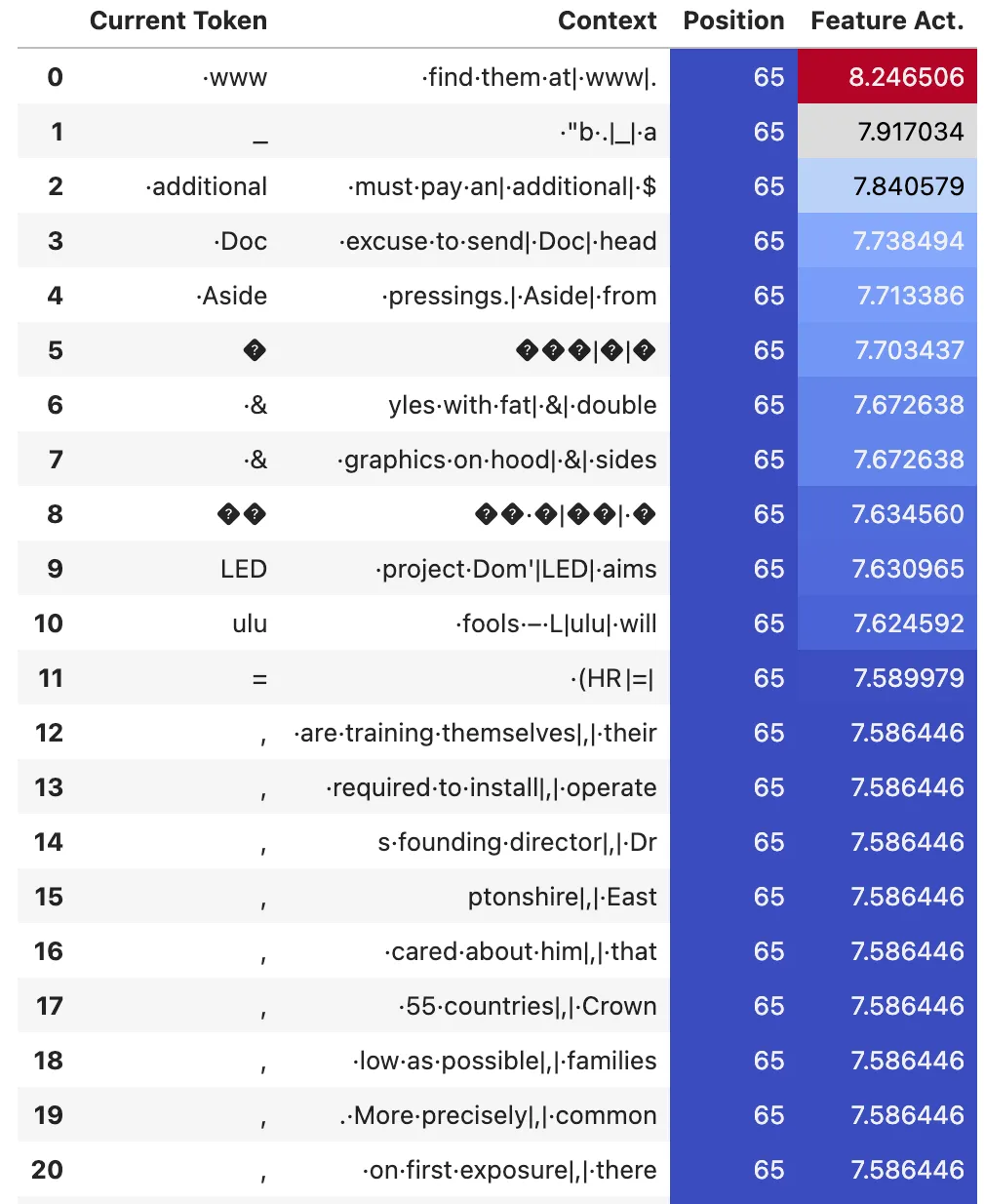
The figure below is intended to describe the tests that I used to find the features that, if removed, would cause the largest change to the attention score between a query and key token. Here I use the decoded activations from the SAE, but delete one of the features when calculating the decoded activations. In the figure, the x axis is the feature ID and the y axis is the attention score (i.e. before softmax etc.) The baseline that most feature IDs fall under corresponds to the fact that most features do not affect the attention score between one given query token and one given key token. The downward spikes in red e.g. at 96, 120 and 173 correspond to features which, if removed, significantly reduce the attention score between these given tokens. Likewise for the blue downward spike at 21. Upward spikes imply increased attention scores if the features are removed.
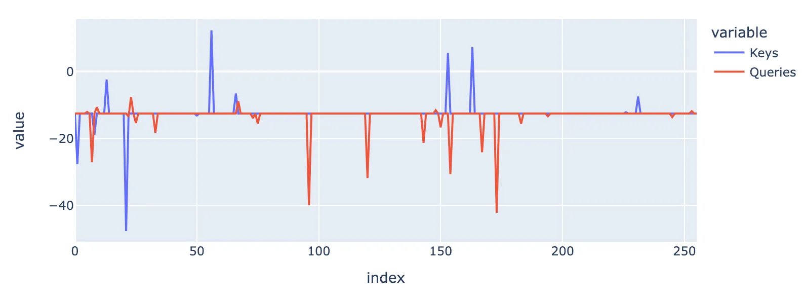
Features that modify attention scores in the above prompt
Induction Heads
Attn-only-2l (L1H6)
Summary
- I trained an SAE on the key and query vectors of the induction head in attn-only-2l.
- Interpretable query features are generally of the form “I am [X] token”, while key features are of the form “I follow [X] token”, where [X] token corresponds to either an individual token, e.g. ·( or a set of related tokens, e.g. ·city ·island ·state ·county
- Despite the fact that there are far fewer features than tokens in the vocab, the ability to perform induction based on the reconstructed key and query vectors remains very good (see figure testing induction on random tokens). I view this as down to the fact that most of the features fire on multiple related tokens and this works out to have enough resolution that induction is therefore performed correctly.
- I can use the features to causally intervene in the logits in such a way that the induction breaks on the token that the feature corresponds to.
- Something to check: do the key features connect to output features from previous token heads in earlier layers?
| Metric | Query | Key |
|---|---|---|
| L0 Norm | 110 | 92 |
| Recovered loss | 99.2% | 88% |
| # Alive features | 1050 | 215 |
| # Features | 8192 | 8192 |
| L1 coefficient | 0.001 | 0.01 |
Typical Query Features
- Query features are typically of the form “I am [X] token”. Here are some examples:
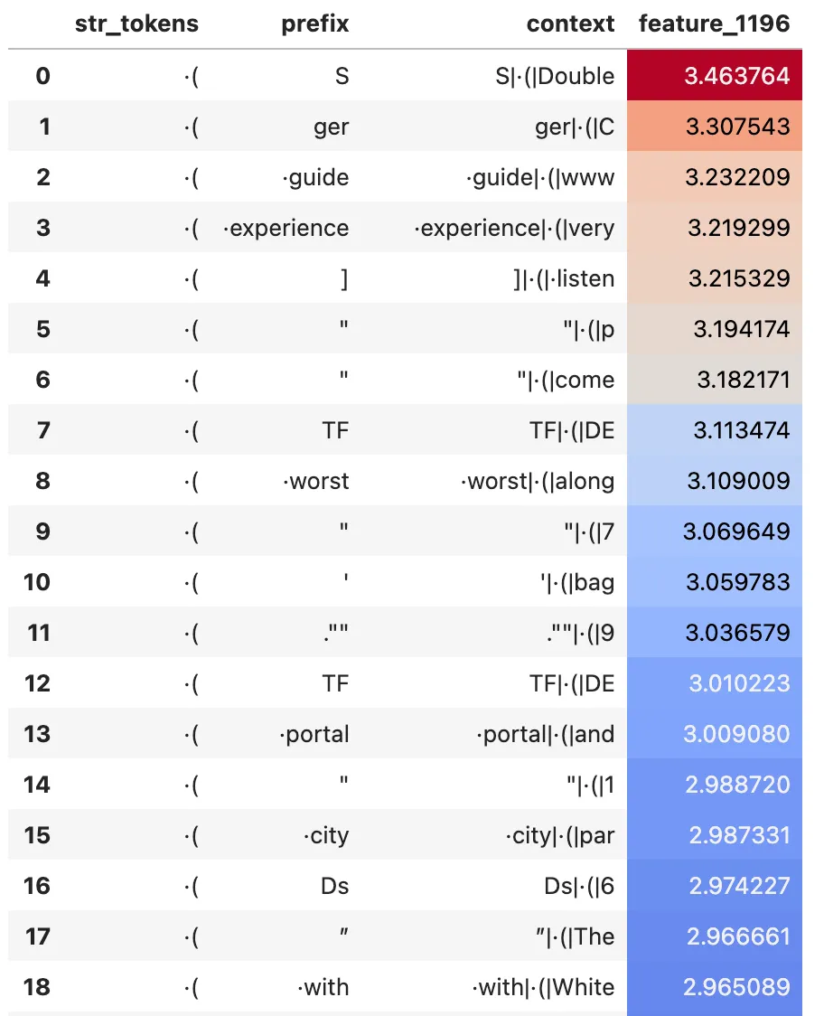
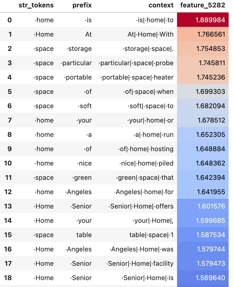
Examples of query features. Left: a monosemantic feature e.g. #1196 fires on ·(. Right a less monosemantic feature e.g. #5282 fires on ·home and ·space
Typical Key Features
Like the attn-only-2l model, key features are typically of the form “I follow [X] token”
Examples of key features. Left: a monosemantic feature e.g. #5965 fires for “I follow [,]”. Right a less monosemantic feature e.g. #919 fires following ·is, ·are and ·become.
Reconstructed Attention Pattern
I tested the performance of the induction head on the task of induction with the reconstructed attention patterns based on the key and query vectors. The prompt I use is
”Mr and Mrs Dursley were perfectly normal. Mr D”
which tokenises into
[Mr] [ and] [ Mrs] [ D] [urs] [ley] [ were] [ perfectly] [ normal] [.] [ Mr] [ D]
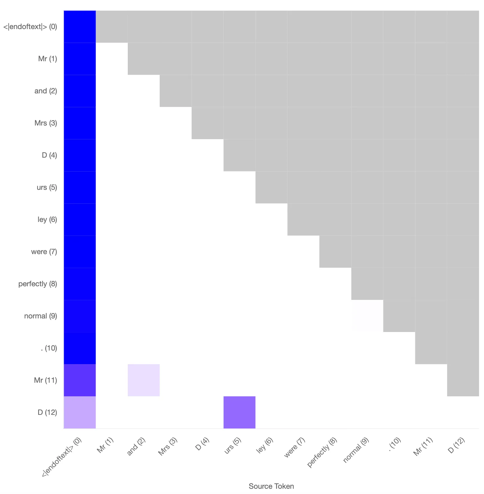
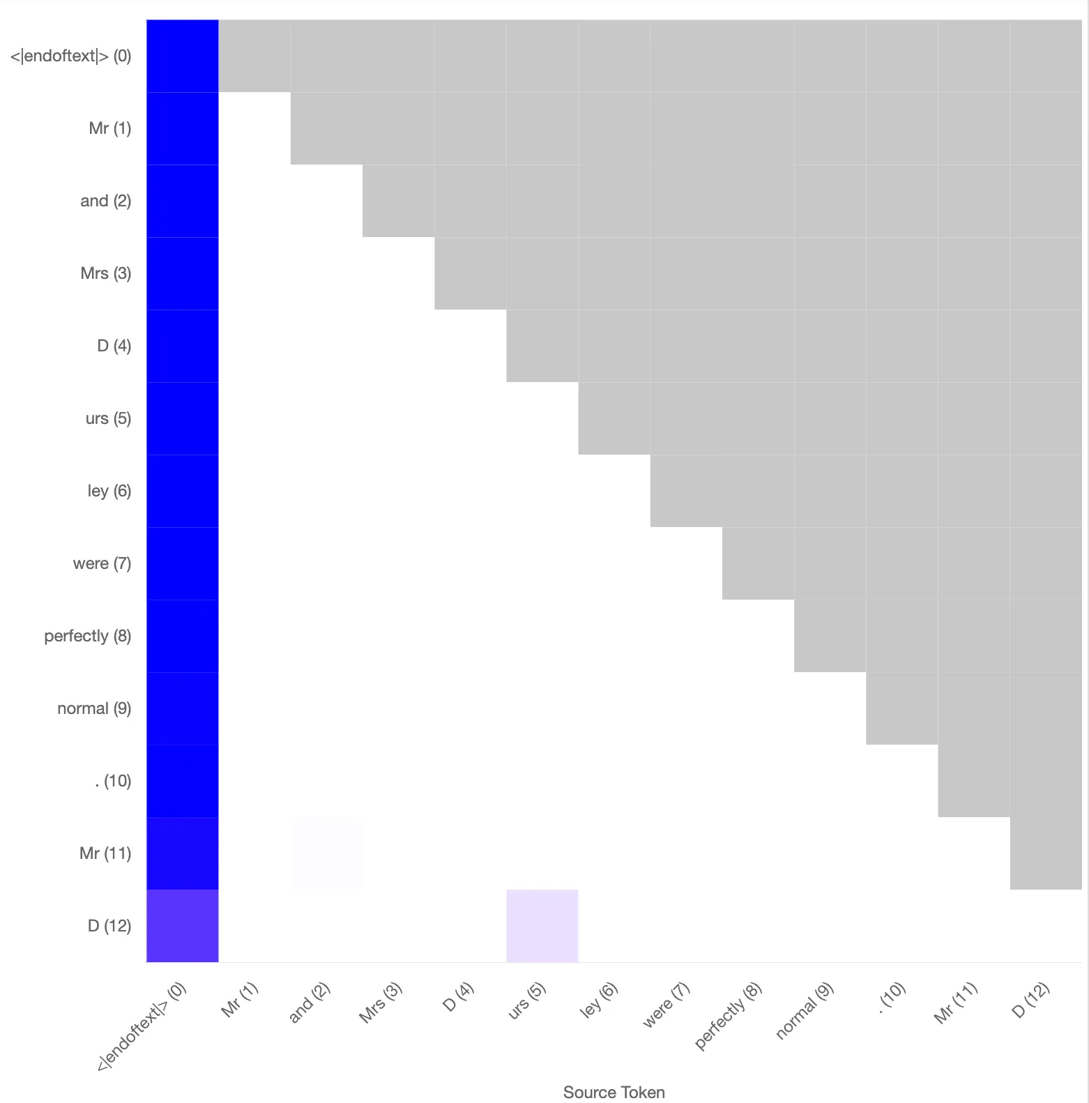
The standard attn-only-2l model uses a previous token head combined with this L1H6 induction head to predict the next token to be [ urs] with a probability of 0.89. Based on the reconstructed attention, one obtains a probability of 0.88. The attention patterns between the model only and the reconstructed pattern based on the SAEs trained on the key and query vectors are qualitatively similar (will quantify).
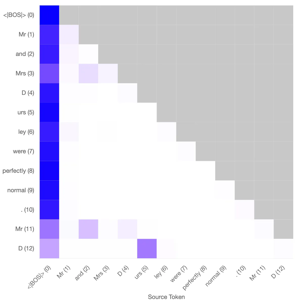
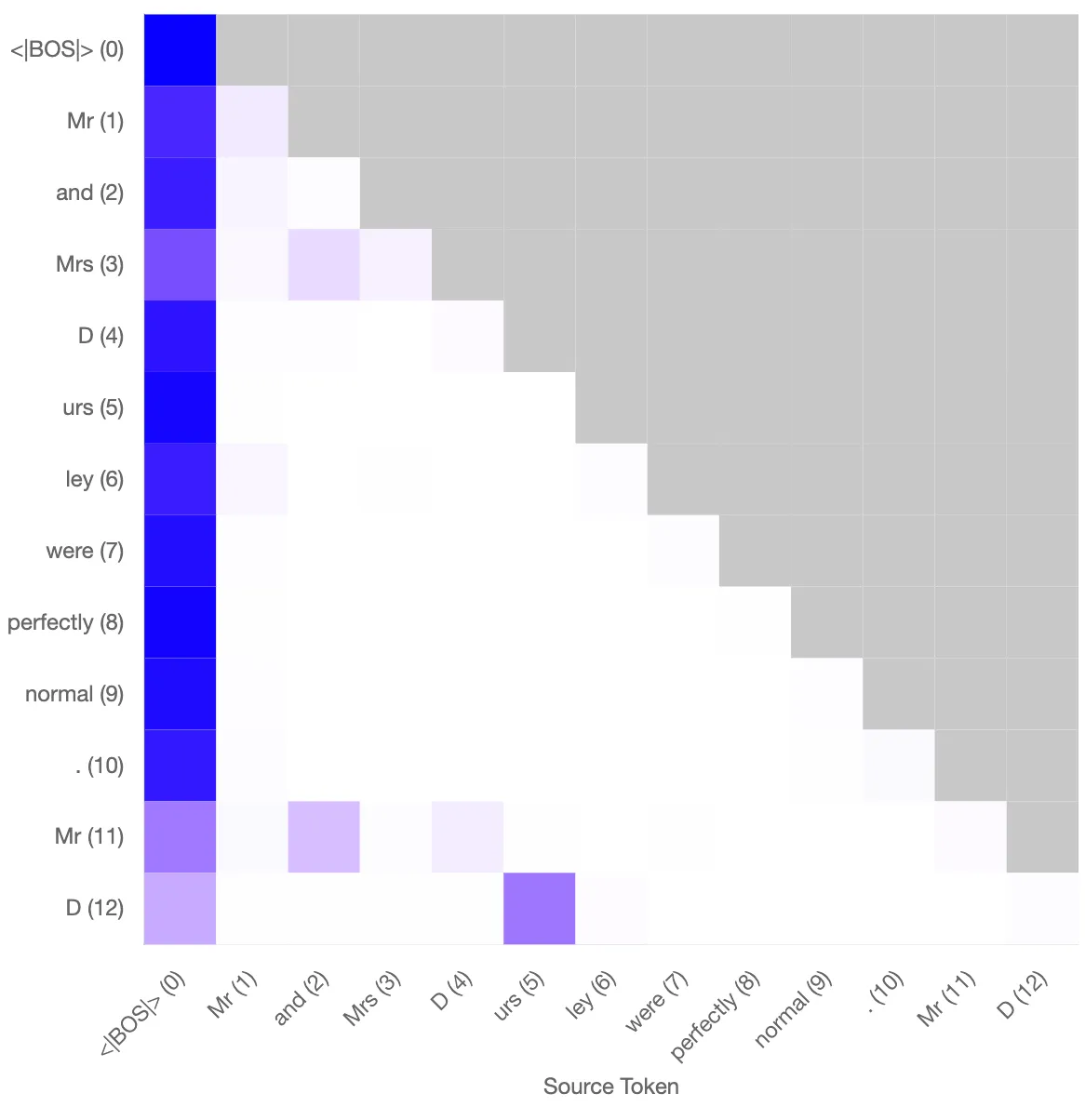
Left: Original attention pattern for the induction head. Probability of “urs” at final token: 0.89. Right: Reconstructed attention pattern using the sparse autoencoder. Probability of “urs” at final token: 0.88.
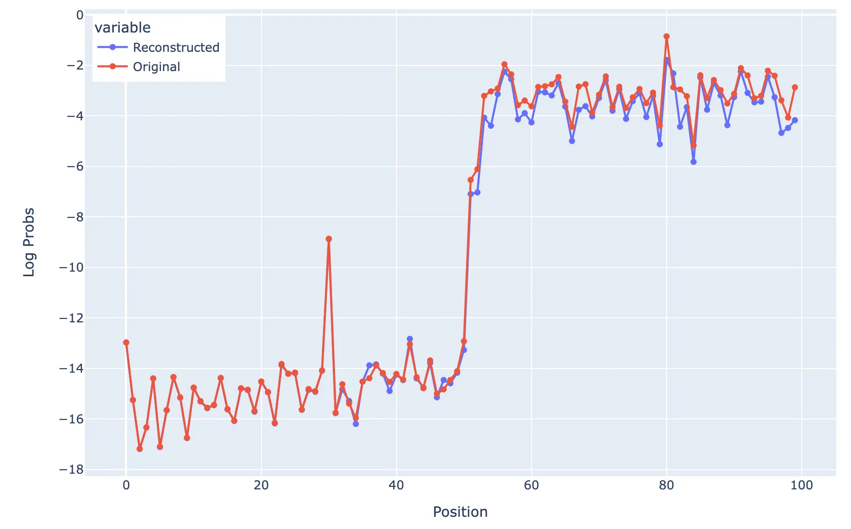
Another test to see how well the model performs the task of induction is to put a prompt of a BOS token followed by a sequence of 50 random tokens and then the same 50 token sequence again. This is a standard setup as used in previous work. Performing this test, the reconstructed Log Probs are slightly lower than the original model, but the model is still clearly capable of performing induction on random tokens, even though we don’t have a feature per token.
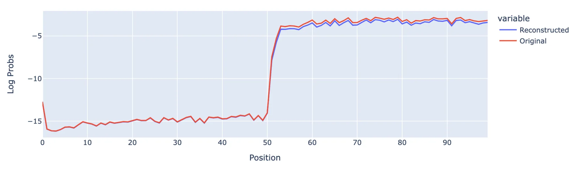
Induction behaviour test using a repeated sequence of 50 random tokens
Impact of ablating features on induction performance (L1H6)
| Reconstructed prob of “urs” predicted at final token | |
|---|---|
| With all features | 0.88 |
| With all features except #5992 | 0.008 |
| Only #5992 | 0.78 |
Using the following prompt:
“Mr and Mrs Dursley were perfectly normal. Mr D”
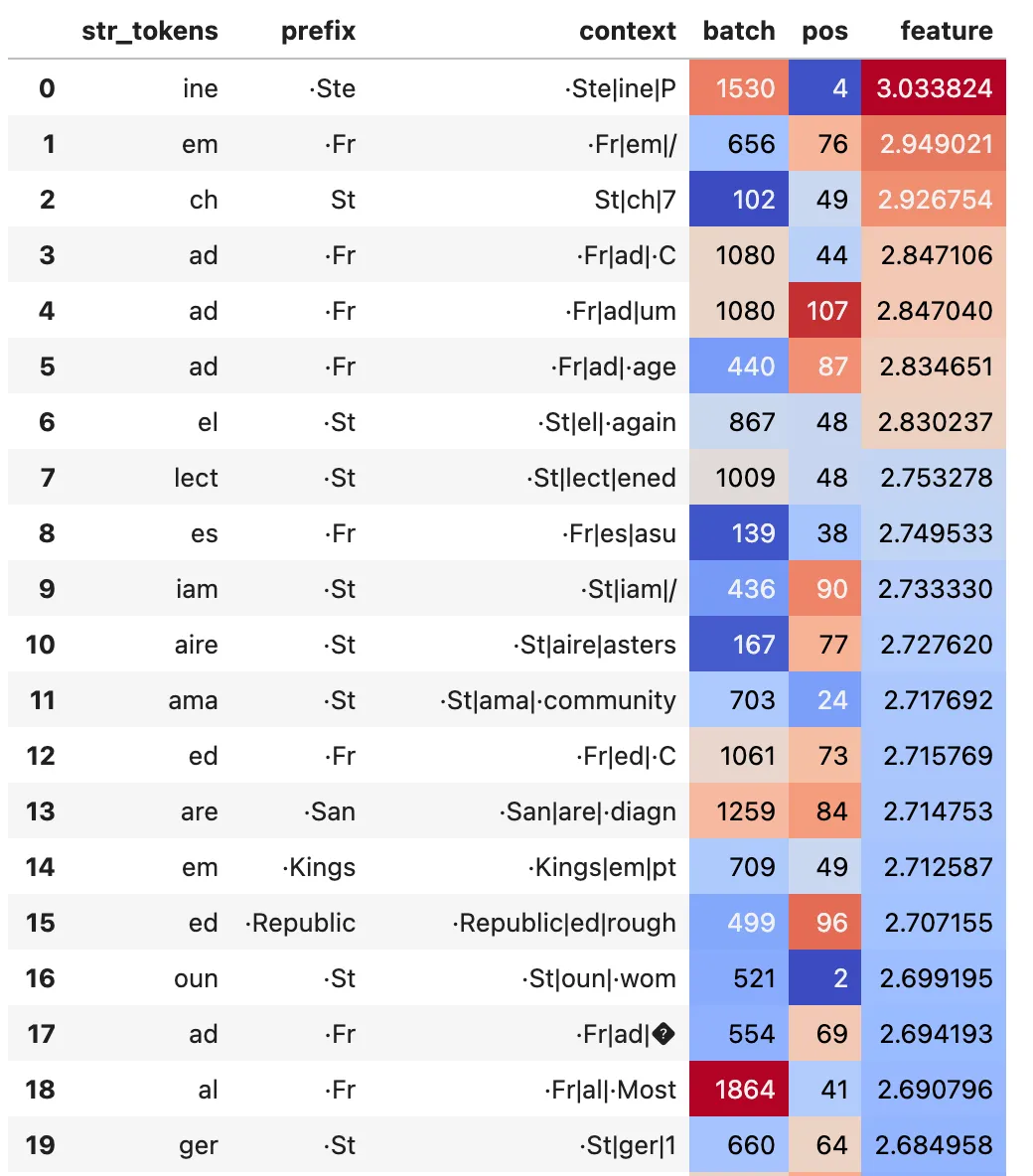
where the final token is “ D”, the distribution of key activations on the first “ D” are below:
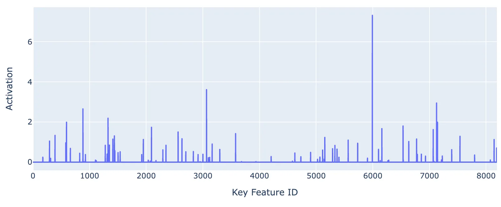
Figure shows key vector SAE activations on token “urs”, where #5992 is the strongest activating feature.
Now I test whether ablating Key Feature #5992 (“I follow [·D]”) breaks induction with random tokens rather than only on the “ urs” token as in the previous example. The setup is as follows:
Prompt consists of BOS + 50 random tokens repeated twice but with token 30 in both repeated sequences set to [·D] Key Feature #5992 (“I follow [·D]”) is subtracted from the key vectors of the first 50 tokens
The main conclusion from this is that the dip at position 81 shows that when feature #5992 is subtracted, the model is much worse at induction specifically with the [·D] token compared to other random tokens
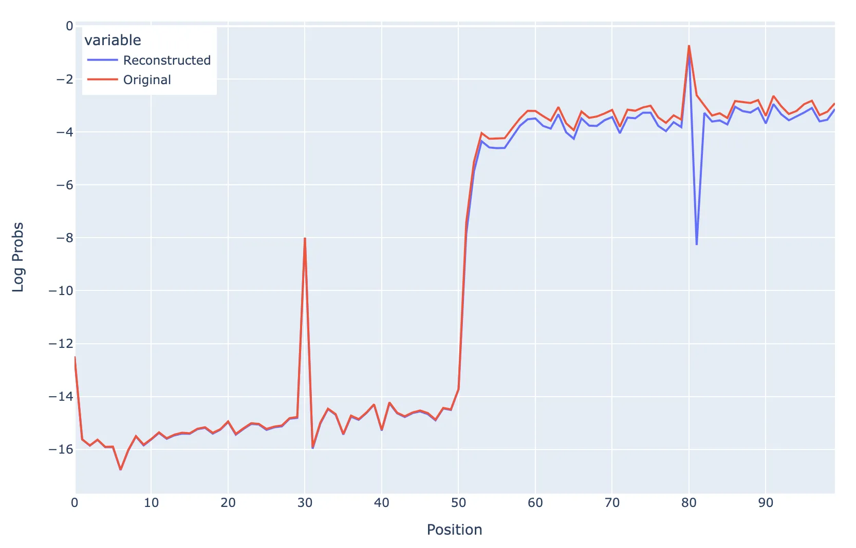
Ablation Test with repeated sequence of 50 random tokens
If you ablate all non-D features at position 31, you get:
Ablating all non-D features at position 31
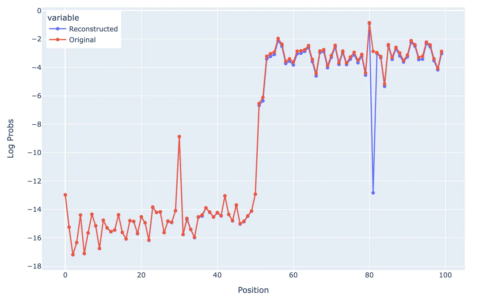
But if you scale up (5x) the magnitude of the I follow D feature at position 31, you get the following picture, that suggests that you can indeed recover a large probability of predicting ·D as long as the magnitude of the activation is large enough.
Ablating all non-D features at position 31 but scaling up the magnitude of the “I follow [D]” feature.
GPT2-small (L5H1)
Summary
| Metric | Query |
|---|---|
| L0 Norm | 91 |
| Recovered loss | 97.6% |
| # Alive features | 800 |
| # Features | 8192 |
| L1 coefficient | 0.01 |
Query and key vector features are similar to the induction head in two-layer model. Induction head behaviour in the attention pattern is somewhat recovered, but with a weaker attention score.
Typical Query Features
Left: Example of monosematic attention head query feature (#417). Right: A somewhat less monosemantic feature
Typical Key Features
Left: Example of monosematic attention head key feature (#2535). Right: A somewhat less monosemantic feature, fires on ·fr and ·st
Reconstructed Attention Patterns
Same prompt of “Mr and Mrs Dursley were perfectly normal. Mr D”, hoping that the final “ D” token attends to the “urs” that followed the “ D” earlier. Induction behaviour is somewhat recovered based on this attention pattern, with a weaker attention fraction on the “urs” token (0.13 vs 0.63 in the original)
Reconstructued attention patterns for the original (left) and modified model using the SAE (right).
The model also performs very well on the 50 random tokens followed by the same 50 random tokens test, but this is affected by the fact that gpt2-small has multiple induction heads. I didn’t have time to investigate it further than this, but this analysis is still limited by the difficulty in training good SAEs with alive interpretable features on gpt2-small.
Name Mover Head in GPT2-small (L9H9)
Summary
These are just brief notes on my experience with L9H9. I did not spend much time on this so do not have firm conclusions.
I trained an SAE on key and query vectors of L9H9, with the idea to see if I could separate out the different functions it performs (name moving in indirect object identification, retrieving name from e.g. Neel Nanda … Mr -> Nanda and converting names to twitter handles). I took a slightly deeper look at the prompt “When Mary and John went to the store, John gave a drink to” as a starting point. Tried with a variety of L1 coefficient and expansion factors. This is more under the banner of exploratory work compared to the previous token heads and the induction heads. Due to the difficulty of having lots of dead features, I ended up looking at a model with 256 learned features (Head is 64 dim space).
- The attention pattern can be approximately reproduced. For instance for the prompt “When Mary and John went to the store, John gave a drink to”, the left plot is the actual attention pattern from the model and the right plot is the reconstructed attention pattern from the decoded key and query vectors. Note that the final token “ to” attends to “ Mary” as in the indirect object identification task.
- Key features that fire on the ‘ Mary’ token are very sparse (one main feature)
- The strongest feature (#32) is clearly a feature that fires on first names.
- Second strongest also fires on certain names
- Query features that fire on the last ‘ to’ token are somewhat less sparse (5 - 6 features).
- Strongest feature (#98) appears to fire when first names have appeared in the context previously.
- 2nd strongest is hard to interpret, but does fire when names are mentioned in the context similar to #98 but further back in the context.
- Could not interpret 3rd strongest
- 4th & 5th strongest look like positional features
- 6th strongest looks like it thinks it’s a one-syllable word (which it is!). Or I’m reading too much into the max activations
- If I compute the (unweighted by activations) dot product between all non-zero features in the key SAE on the token ‘ Mary’ and the query token ‘ to’, the strongest combination is the one between the key feature #32 (‘I am a name’) with query feature #98 (‘I followed a name’). This is also true for both ‘ John’ tokens so I need to investigate further why it attends more strongly to ‘ Mary’ in this context.
- Somewhat separate to these points, features in the key vector SAE include positional features that look similar to the previous token head features
- I did not find features related to understanding “Neel Nanda …. Mr” -> Nanda or related to twitter handles.
Method used to train sparse autoencoders
- I trained with a setup matching that of Anthropic’s paper “Towards Monosemanticity”, except applied to different model components.
- I mainly trained with Neel’s c4-tokenized-2b and also briefly experimented with the Pile and OpenWebText
- I originally wrote my own method (based on Neel’s code) to train the models. It worked fine initially, but given the two-week time period, I decided to use the open-source one available at https://github.com/ai-safety-foundation/sparse_autoencoder/tree/main to allow me to focus on actual training and experimentation with the attention heads. I made a series of customisations to this code including making it work on the concatenated attn-z layer, single attention heads, pre-computing activations separate to training the SAE, writing and reading pre-computed activations and fixing a few bugs.
- About halfway through the research sprint, I reached the point where it would be significantly more efficient to write my own code from scratch as there are now several features that I’d like to implement in my own way. These will include:
- Pre-computed activations. These result in such a significant speed-up (2x - 3x) that I’d consider them a vital component of doing proper hyperparameter sweeps
- Proper logging of the training process, e.g. density of features, live views of how each feature changes over time by max activations. I think this is useful to understand how the hyperparameters change things.
- Proper handling of restarts
- Allow for optimising for different quantities rather than loss based on mean squared error, e.g. attention scores/pattern.
- The re-sampling helped in some places and didn’t help in others. Anecdotally, it felt like it tended to help more clearly in models trained on the MLP layers or on the concatenated attn-z layer. In the places where it didn’t help, the features died very soon after each re-sampling event. This is something I want to investigate further properly as it seems at the core of why it was difficult to train on attention heads of gpt2-small in the first place.
General comments regarding training SAEs on attention heads
- I often got lots (~85%) of dead features with attention heads in GPT2-small compared with smaller 1L and 2L models, in which it was easy to have close to ~100% alive features. It appears to be difficult to avoid this without significantly increasing the L0 norm to ~500. This is the biggest methodological problem I’d try to solve in future work.
- I found that a high L0 is sometimes not a problem for interpretability because it’s possible that only 1 or 2 features contribute significantly to the function that is taking place. I discussed this explicitly with the induction head in attn-only-2l. This is related to the general question of which metrics are useful to consider in deciding how good the SAE is. But I’d just make the point here that if you have 1 – 3 features that activate strongly and 20 that activate weakly, then it might still be reasonably interpretable and easy to casually intervene on. It just depends on the distribution of the activations of the features on the token you are looking at. I’d also note here that it’s definitely possible that the high L0 norm might just be a consequence of not enough training activations. Due mainly to time constraints in the two week window, I worked mainly with 200m - 400m activations. Perhaps training to 2b kills all the weakly activating features. The Anthropic team suggests that longer training improves interpretability.
- It’s a much better idea to write activations to disk and then read. I tried this for one of the heads and it resulted in a 2x - 3x speedup. I have been running my models on paperspace and did not easily figure out a way to allow for larger storage of several 100 Gb (maxed out at 50Gb) so was unable to fully generalise this. I’d consider this a necessity for properly exploring this topic in the future.
- I haven’t fully thought this through, and need to test it properly, but it’s possible that you need to be careful with how BOS tokens are considered in the training data for the SAEs on attention heads. A problem that could arise is that the query vectors do not know they should attend to the BOS token unless it’s usually at position 0 in the SAE training set.
- Key vectors seem anecdotally more difficult to train than the query vectors. I didn’t have time to properly study this. One example that hints at this intuition are the feature density diagrams for the previous token head in attn-only-2l. One can see that the best query model ended up with no dead features, but the best key model ended up some dead features. Another example is that shows that there is at least a difference between the two is the fact that the L1 coefficients that ended up being best for the gpt2-small induction head were 0.001 for the query vectors and 0.01 for the key vectors
Future Directions
- Investigate multiple induction heads in gpt2-small further – I ran out of time to properly explore multiple heads. Exploratory experiments involving training SAEs on the query vectors of L5H1 and L5H7 heads show no obvious difference between the query and key features of each head. This investigation could be combined with non-SAE based investigation along the lines of, e.g. does each induction head perform induction better for a subset of tokens?
- I think attention head superposition is also a logical next step following on from looking at individual attention heads. I have already trained an SAE on the concatenated z output of all attention heads in the first layer of gelu-2l to search for superposition. I did not find any, but should possibly look at a larger model or later layer to search for such superposition.
- Try on some random attention heads in gpt2-small. I tried on a random head in attn-only-2l, but nothing jumped out immediately and I didn’t get enough time to properly go through the results.
- It would also be interesting to explore using only part of the data distribution rather than the full data distribution as used in Arthur Conmy’s recent paper. This might facilitate more deliberate function finding of the heads.
- I think it would be useful to explore trying to minimise something other than the loss, for instance the recovered attention pattern, attention scores or performance on a standard task e.g. induction or name mover. This might draw out the features that are able to perform a particular task more strongly.
- Train the SAEs for longer. I mainly focused on interpretability of features and exploring different types of attention heads in these two weeks, but with more time could train these and this might improve the metrics.